

My Research Themes
I am primarily interested in understanding stellar spectroscopic variability, with the ultimate goal of mitigating its impact on radial velocity (RV) measurements and enabling the detection and characterization of Earth-mass planets orbiting Sun-like stars. To help meet this goal, I use our nearest star, the Sun, as a laboratory to understand how convective motions and other magnetic phenomena in the solar atmosphere create RV variability several times larger than the 10 cm/s RV semiamplitude of the Earth.
A full list of my publications is available here and as a SciX library. My works are generally accompanied by software releases or worked examples. The relevant GitHub repos are linked through the icons next to the section headers.
 Simulating Granulation-driven Variability
Granules are convective cells in the photosphere of stars. In the Sun, they appear as irregularly shaped bright regions surrounded by darker regions known as intergranular lanes. Many granules can be seen in the accompanying animation, which shows a patch of the solar surface observed by the Daniel K. Inouye Solar Telescope (DKIST). The convection in these cells creates a source of persistent RV noise on the order of several tens of cm/s. To understand the precise effects of these granules on RV surveys, I use high spectral resolution observations of the Sun to create synthetic spectra with realistic perturbations from granules. This tool, the GRanulation And Spectrum Simulator (GRASS), is available on GitHub.
You can view a short summary of my 2022 paper presenting GRASS on this poster. In my 2024 paper, I show that variations in the shapes of individual lines can be an important tool for removing variability in RV measurements.
🌘 Modeling Solar Eclipse Observations
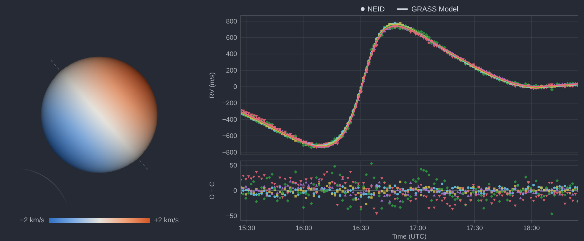
During the annular solar eclipse of 2023 October 14, the NEID spectrograph at the WIYN telescope observed the Sun as a star while the Moon crossed the solar disk. Because the Sun rotates, the Moon blocks first one limb and then the other, so the disk-integrated radial velocity swings by over a kilometer per second: the solar counterpart of the Rossiter–McLaughlin effect seen when planets transit their stars. The eclipse is a rare chance to test line-shape models against the Sun with part of its disk masked out. Led by Elizabeth Gonzalez, we extended GRASS to simulate eclipse observations line by line and compare them to the NEID data; the paper (Gonzalez et al., in prep.) is forthcoming.
 Modeling Absorption Line Formation
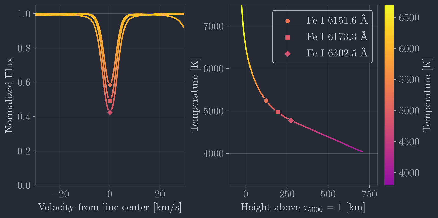
Absorption lines do not form at a single depth in a stellar atmosphere. Each wavelength across a line escapes from a different layer: the core of a strong line samples cool gas high in the photosphere, while its wings and the surrounding continuum sample hotter gas below. Knowing where each part of a line forms is what makes line shapes a probe of how velocities change with height. FormationTemps.jl wraps Korg.jl to compute synthetic spectra and the formation temperature at every wavelength from stellar parameters and a linelist, integrating rotation and turbulence over the stellar disk instead of approximating them with a convolution that breaks down at high spectral resolution. I present the method in my 2026 ApJ paper.
The accompanying widget shows one Fe I line profile, colored by formation temperature. Hover over or drag along the profile to pick a wavelength; the atmosphere panel then shows the temperature and height at which that wavelength forms, along with the contribution function behind it.
 Inferring Convective Velocities
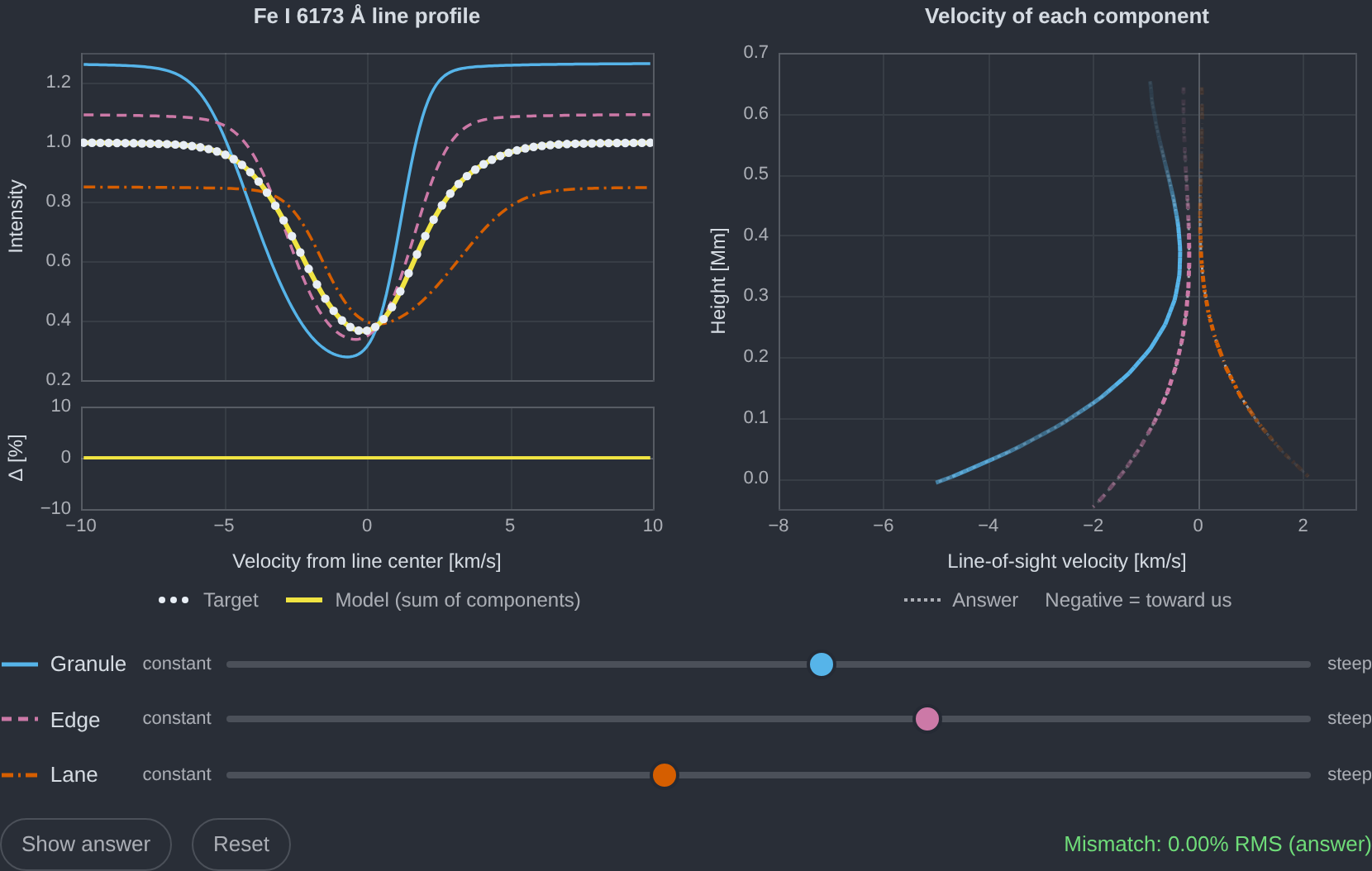
Granulation perturbs the shapes of absorption lines. By writing down a forward model that can perform the radiative transfer accounting for moving layers of the stellar atmosphere, it is possible to infer the velocity stratification of the atmosphere directly from observed spectra. This work is currently in progress, but you can find a preview of the radiative transfer forward modeling in my 2026 ApJ paper on calculating formation temperatures for stellar spectra.
 Solar Center-to-limb Variability

In addition to granulation, other features in the atmospheres of stars can cause large RV anomalies. These phenomena include sunspots, magnetic network, and plage, among others. To study how these regions and the altered velocity flows therein manifest in RV measurements, I use data from the Solar Dynamics Observatory (SDO) to classify these different regions, and then calculate their contribution to the observed suppression of convective blueshift as a function of limb angle. I found that this suppression is not always a suppression: toward the limb, plage and network are blueshifted relative to the quiet Sun, enhancing the convective blueshift. You can read the paper in ApJ.
The accompanying widget opens on histograms of each region’s velocity in SDO images taken every four hours from 2012 to 2015, for one limb-angle bin that the slider below it changes. Its CLV Curves view plots each region’s mean velocity against limb angle, and its Sun view shows how one of those images is classified; hover over the disk to name the region under the pointer. Click a region in the legend to isolate it in every view.
📡 SETI
As part of Jason Wright’s graduate course in SETI, I co-authored a paper in which we searched for radio signals transmitted by a hypothetical probe using the solar gravitational lens to aid in communication across interstellar distances (Tusay and Huston et al. 2022). The observations conducted for this work targeted the antipode of the Alpha Centauri system. In a follow-up work (Palumbo, Wright, & Huston 2023), we show that over 1500 additional archival observations conducted with the Green Bank Telescope were fortuitously pointed at the antipodes of stars within 100 parsecs of the Sun. To facilitate the analysis of these observations, we have tabulated the drift rates and other relevant parameters for searching these data for artificial signals.
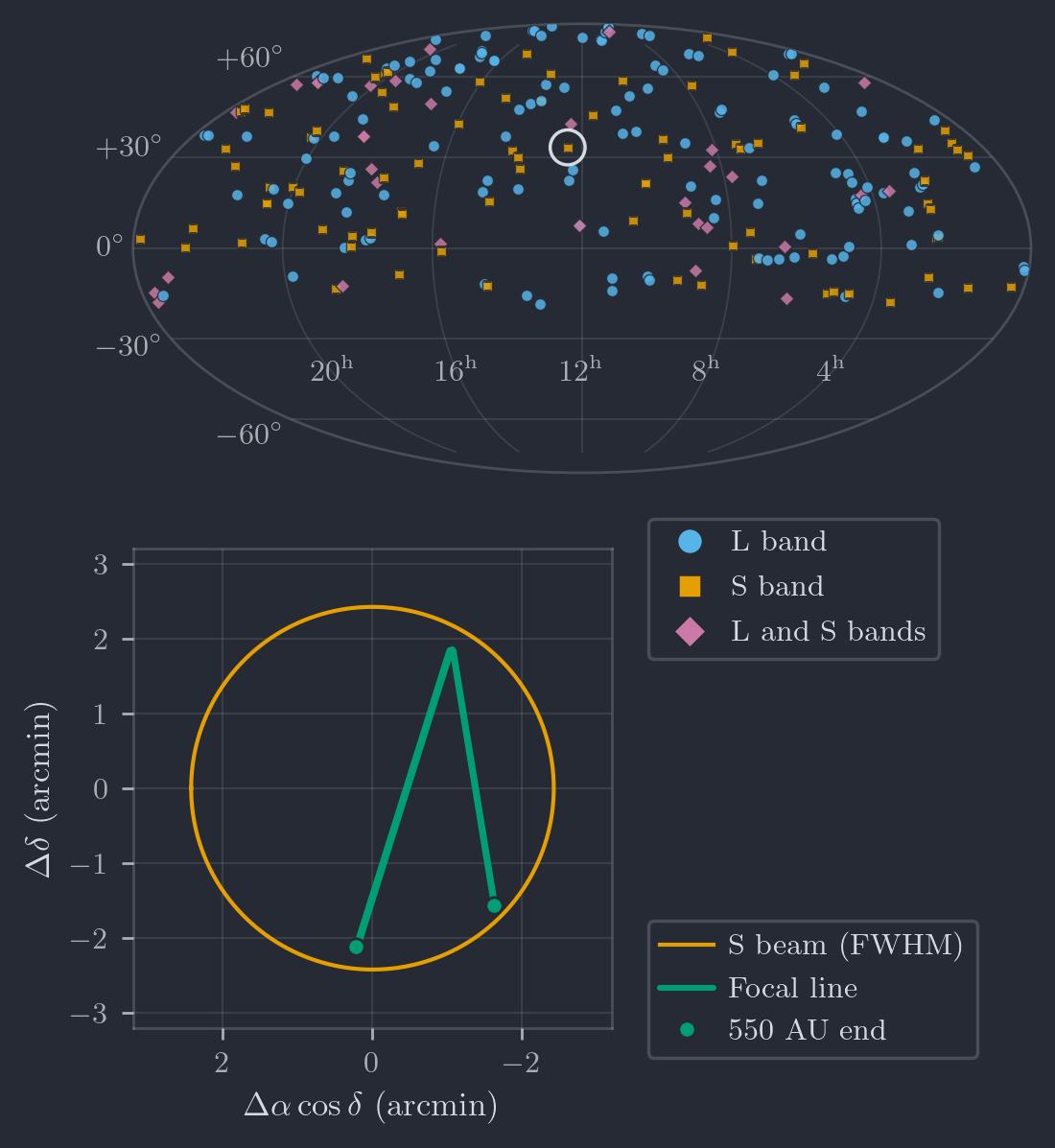
A relay probe using the Sun as a gravitational lens would sit at least 550 AU from the Sun, on a focal line in the part of the sky opposite the star it communicates with. The accompanying widget maps the 253 Breakthrough Listen targets, observed in 709 scans, whose beams happen to contain part of such a focal line for one of 257 stars within 100 pc, marked by the bands they were scanned in. Click or tap a marker to see that target’s beams and each distinct focal line in them. The dot marks a line’s 550 AU end, which shifts with Earth’s orbit between observing dates while the far end barely moves. Because only Earth’s motion sets the drift rate of a signal from such a probe, these data can be searched far more deeply than a search over unknown drift rates allows.
The article is published in Research Notes of the AAS; a PDF of this work and a supplemental Jupyter Notebook are available on GitHub.