Basic Usage

The most basic use case of GRASS is generating time series of synthetic spectra and measuring apparent velocities. These can both be done in only a few lines of code.

Generating Synthetic Spectra

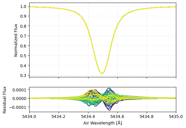
The simplest use case for GRASS is the generation of time series of synthetic spectra. This can be done in only a few lines of code. The following example generates 25 spectra consisting of a single line at 5434.5 Angstroms. By default, the temporal spacing of the spectra is 15 seconds.

using GRASS
using Statistics

# PythonPlot comes from the default environment, not from GRASS's dependencies
import PythonPlot
const plt = PythonPlot.pyplot
const mpl = PythonPlot.matplotlib

# parameters for lines in the spectra
λrest = 5434.5
lines = [λrest]     # array of line centers in angstroms
depths = [0.75]      # continuum-normalized depth of lines
resolution = 7e5     # spectral resolution of the output spectra
spec = SpecParams(lines=lines, depths=depths, resolution=resolution)

# specify number of epochs (default 15-second spacing)
disk = DiskParams(Nt=50)

# synthesize the spectra
wavelengths, flux = synthesize_spectra(spec, disk)

# get the residuals
resid_flux = flux .- mean(flux, dims=2)

# get a colormap for time
cmap = plt.get_cmap("viridis")
colors = cmap(range(0, 1, length=disk.Nt))
norm = mpl.colors.Normalize(vmin=15, vmax=15*disk.Nt)
smap = mpl.cm.ScalarMappable(norm=norm, cmap=cmap)

# plot the result; the axis array comes back as a Python object, so it is indexed from 0
fig, axs = plt.subplots(nrows=2, ncols=1, height_ratios=[3,1], sharex=true)
ax1 = axs[0]
ax2 = axs[1]
for i in 1:disk.Nt
    xs = wavelengths
    ys1 = view(flux, :, i)
    ys2 = view(resid_flux, :, i)
    ax1.plot(xs, ys1, c = colors[i, :])
    ax2.plot(xs, ys2, c = colors[i, :])
end
ax2.set_xlabel("Air Wavelength [Å]")
ax1.set_ylabel("Normalized Flux")
ax2.set_ylabel("Residual Flux")
ax1.grid(ls = ":", alpha=0.5)
ax2.grid(ls = ":", alpha=0.5)
ax1.set_xlim(λrest - 0.5, λrest + 0.5)
fname = joinpath(GRASS.moddir, "docs", "src", "assets", "spectrum.png")
plt.savefig(fname, bbox_inches="tight")
plt.show()

Measuring Velocities

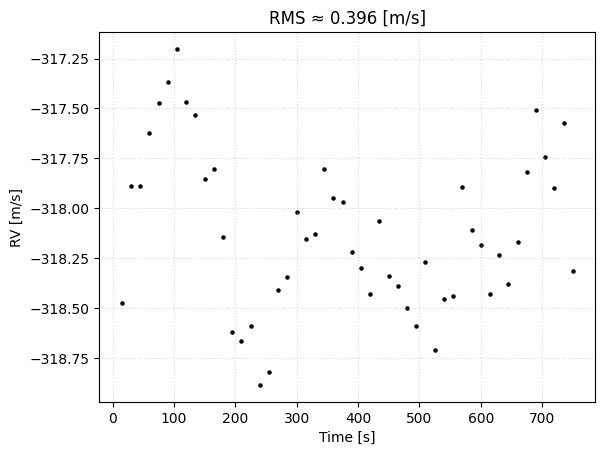
GRASS wraps the EchelleCCFs package to measure apparent Doppler velocities from spectra.

# generate a velocity grid and compute the cross-correlation function
vel_grid, ccf = calc_ccf(wavelengths, flux, spec, normalize=true)

# measure radial velocities and uncertainties from the ccfs
rvs, sigs = calc_rvs_from_ccf(vel_grid, ccf)

# measure an rms
rms = calc_rms(rvs)
rms_string = string(round(rms, digits=3))

# plot the RVs
plt.scatter(15 .* collect(1:disk.Nt), rvs, c="k", s=5)
plt.xlabel("Time [s]")
plt.ylabel("RV [m/s]")
# plt.xlim(0, 15 * disk.Nt + 1)
# plt.ylim(minimum(rvs) - rms, maximum(rvs) + rms)
plt.title("RMS ≈ $rms_string [m/s]")
plt.grid(ls = ":", alpha=0.5)
fname = joinpath(GRASS.moddir, "docs", "src", "assets", "rvs.png")
plt.savefig(fname, bbox_inches="tight")
plt.show()

Measuring Bisectors

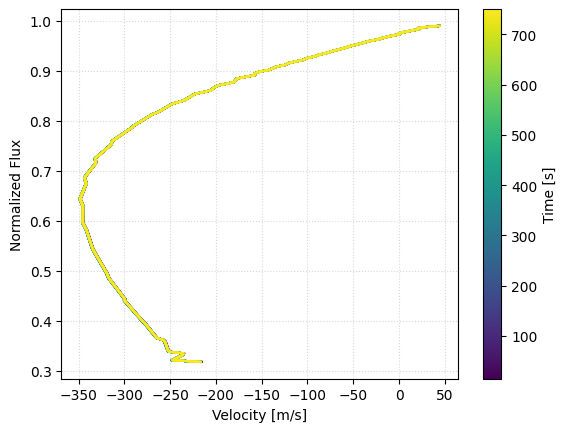
GRASS wraps the EchelleCCFs package to measure apparent Doppler velocities from spectra.

# measure bisectors
bis_wavs, bis_flux = calc_bisector(wavelengths, flux, nflux=200)

# cut off the bottom-most noisy measurement
bis_wavs = bis_wavs[2:end, :]
bis_flux = bis_flux[2:end, :]

# convert to from a wavelength to a velocity scale
bis_vels = GRASS.c_ms .* (bis_wavs .- λrest) ./ λrest 

# plot it 
for i in 1:disk.Nt
    xs = view(bis_vels, :, i)
    ys = view(bis_flux, :, i)
    plt.plot(xs, ys, c=colors[i,:])
end
plt.xlabel("Velocity [m/s]")
plt.ylabel("Normalized Flux")
plt.colorbar(smap, label = "Time [s]", ax=plt.gca())
plt.grid(ls = ":", alpha=0.5)
fname = joinpath(GRASS.moddir, "docs", "src", "assets", "bisectors.png")
plt.savefig(fname, bbox_inches="tight")
plt.show()

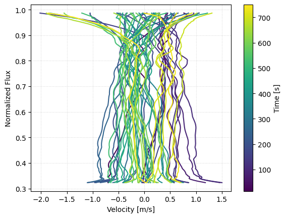
We can also examine the mean-subtracted bisectors to better see the temporal variability in line shape created by granulation.

# now measure the means
mean_bis_wavs = mean(bis_wavs, dims=2)
mean_bis_vels = mean(bis_vels, dims=2)

# get residuals
resid_bis_wavs = bis_wavs .- mean_bis_wavs
resid_bis_vels = bis_vels .- mean_bis_vels

# smooth them
n = 10
resid_bis_wavs_smooth = moving_average(resid_bis_wavs, n)
resid_bis_vels_smooth = moving_average(resid_bis_vels, n)
bis_flux_smooth = moving_average(bis_flux, n)

# plot it
for i in 1:disk.Nt
    xs = view(resid_bis_vels_smooth, :, i)
    ys = view(bis_flux_smooth, :, i)
    plt.plot(xs, ys, c=colors[i,:])
end
plt.xlabel("Residual Velocity [m/s]")
plt.ylabel("Normalized Flux")
plt.colorbar(smap, label = "Time [s]", ax=plt.gca())
plt.grid(ls = ":", alpha=0.5)
fname = joinpath(GRASS.moddir, "docs", "src", "assets", "bisector_resids.png")
plt.savefig(fname, bbox_inches="tight")
plt.show()